Loading BasketAI...
Loading BasketAI...

The final sales forecasting model uses a Deep Neural Network to predict the sales. It has been built using NeuralProphet, which is a Neural Network based PyTorch implementation of FBProphet - the popular forecasting tool developed by Facebook. The model uses past 1.5-2 years of sales data, to forecast n days into the future. The model can produce both single step and multi step-ahead forecasts. At the moment, NeuralProphet builds models univariately, therefore it can only forecast one SKU at a time.
Data pre-processing and filling in missing sales data
Data regularization using a savgol filter

Moving window forecast (Used later as an input feature and future regressor)
Fast to train three-layer deep neural network
A huber loss function along with automatic batch size and epoch size selection

Insights into trend, weekly seasonality, business cycles, yearly seasonality and impact of other regressors like selling price variation
Select how many days into the future to predict
Select input features and future regressors like selling price
Select yearly seasonality for particular SKUs
Select in-built holiday or event variation for particular SKUs
I started out by familiarizing myself with the dataset. This involved visualizing the data and trying to figure out various trends or seasonalities within the data. I carried out the forecasting using a train/test split of 80/20. Before moving onto the complex forecasting models involving machine learning, I tried out various simpler forecasting models:
Naive Forecasting - Assumes that the next expected point is equal to the last observed point
Simple Average Forecasting - Forecasts the expected value equal to the average of all previously observed points
Moving Average Forecasting - Uses window of time period for calculating the average
Simple Exponential Smoothing - Forecasts are calculated using weighted averages where the weights decrease exponentially as observations come from further in the past, the smallest weights are associated with the oldest observations.
Holt’s Linear Method - A method that takes into account the trend of the dataset is called Holt’s Linear Trend method.
Holt-Winters Method - This method comprises the forecast equation and three smoothing equations — one for the level, one for trend and one for the seasonal component.
SARIMAX - ARIMA models aim to describe the correlations in the data with each other. An improvement over ARIMA is Seasonal ARIMA. It takes into account the seasonality of the dataset just like Holt’ Winter method.
Based on each model’s predictions after implementation, I put these 7 methods into two Categories -
Long-term Accuracy - [Methods 1,2,3 and 4] These predictions do not have daily variance and the prediction for each day is very inaccurate. However, over a week or a month, the values provide a very accurate description of the sales. These models performed better with the current error metrics (RMSE and SMAPE).
Short-term Accuracy - [Methods 5,6, and 7] These predictions have a lot of variance and can very accurately predict a day’s sales. However, when they do not predict the sales accurately, the deviation from the actual values is much higher than Category 1, causing a much higher RMSE and SMAPE score in the end.
I then tried out FBProphet, a popular forecasting library created by Facebook. This is an efficient and accurate method to not only create time-series forecasting models, but also get insights into the various seasonality and trend patterns.
After playing around with different parameters and hyperparameters, I implemented an FBProphet Forecasting model as well. The results were similar to those of the Holt-Winters model. I noticed that this model performed really well on some of the products but extremely badly on other products. After analysis, it seemed to be getting the trend wrong in cases where the predictions were bad.
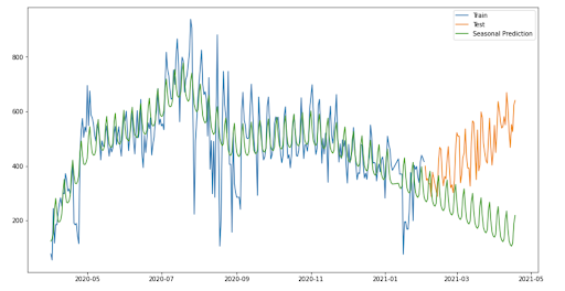

Till now, the moving average prediction model was giving the best results in terms of RMSE and SMAPE. Even though it didn’t have daily accuracy, it always got the trend correctly.
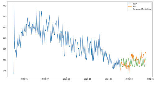
So, I combined the variance predicted by FBProphet with the trend predicted by the moving average model. The resulting model performed extremely well, and also gave the best results in terms of RMSE and SMAPE.

Weekly predictions: I resampled the data to have a frequency of 7 days. However, there wasn’t enough data to make very accurate predictions, and all models worked poorly on this resampled data.
Gaussian Smoothing: I tried various smoothing methods and parameters within those methods to normalize the data, but the models seemed to perform better without the smoothing.
Artificial Variance: All the predictions in methods 1-7 had some or no amount of variance, and usually dampened towards the end. The actual data has a lot of variance, therefore I created a formula to add artificial variance based on the variance of the previous window.
y_hat_new = (y_hat - y_hat.mean())*sqrt(sigma/sigma_hat) + y_hat.mean()
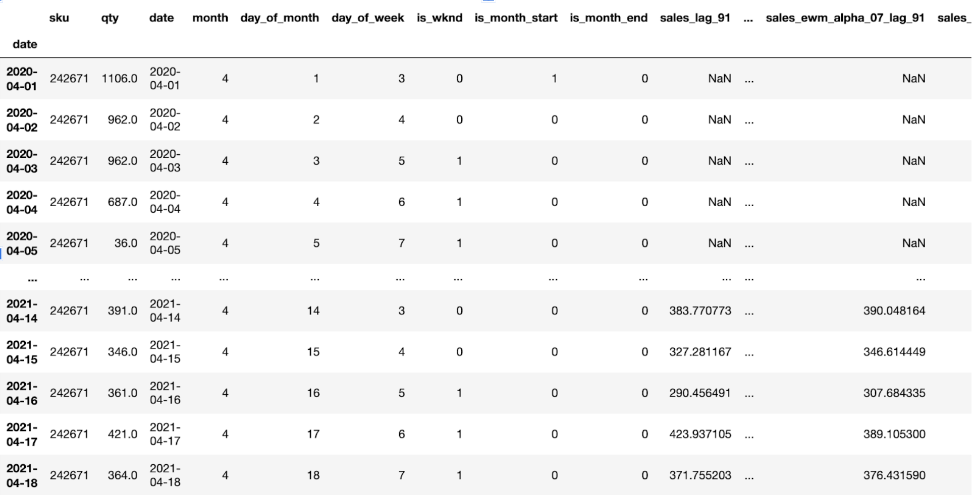
I spent a lot of this week on feature-engineering. These new features included a sales roll of 7, 30, and 180 days. It also included lag features of various lengths. I added new time-series features of one-hot values like week-start, week-end, month-start, month-end, day of the month, day of the week, etc.
I started out with a basic univariate single time-step LSTM RNN Model. Long Short Term Memory networks – usually just called “LSTMs” – are a special kind of RNN, capable of learning long-term dependencies.
In order for the model to learn features from the past as well the future, I converted this basic LSTM into a bidirectional model. I also implemented a multivariate LSTM, which can take Multiple Parallel Series as input. Finally, I converted this model to a multi-step vector output model, which can predict more than one day in the future.
I added the capability of predicting n-days in the future at a time, instead of the entire testing data. I also added the capability of comparing cumulative results instead of daily results; these would be more accurate and helpful in use cases where only the total amount is required.
I also created a simple new formula to optimize the moving average prediction by tuning the size of the rolling window:
window = 14 + int(test_period/7))
This variability on the window length tuned to the specific forecast period gave better results.
The model reached an average accuracy >90% for many of the SKUs over 50 iterations, and an accuracy of >85% for almost all SKUs for the cumulative error. The 7 day daily errors were also mostly in the 80-95% range, although the 30-day daily and 90-day daily predictions were frequently below 80%.
            import pandas as pd
            import numpy as np
            from neuralprophet import NeuralProphet
            import matplotlib.pyplot as plt
            from scipy.signal import savgol_filter
            import plotly.graph_objs as go
            from plotly.offline import init_notebook_mode, iplot
            df_year1 = pd.read_csv('chennai_year1.csv', header=0, low_memory=False)
            df_year2 = pd.read_csv('chennai_year2.csv', header=0, low_memory=False)

            df_year1['date'] = pd.to_datetime(df_year1.order_delivery_date_id,format='%Y%m%d')
            df_year1.index = df_year1.date
            df_year1['sku'] = df_year1.source_sku_id
            df_year1['qty'] = df_year1['sum']
            df_year1['sales'] = df_year1['sum(2)']/df_year1['sum']

            df_year2['date'] = pd.to_datetime(df_year2.order_delivery_date_id,format='%Y%m%d')
            df_year2.index = df_year2.date
            df_year2['sku'] = df_year2.source_sku_id
            df_year2['qty'] = df_year2['sum']
            df_year2['sales'] = df_year2['sum(2)']/df_year2['sum']

            df_year1 = df_year1.drop(columns=['order_delivery_date_id', 'source_sku_id', 'sum', 'sum(2)', 'date'])
            df_year2 = df_year2.drop(columns=['order_delivery_date_id', 'source_sku_id', 'sum', 'sum(2)', 'date'])

            data = pd.concat([df_year1,df_year2])

            data
            # Selects random SKU with large number of sales
            def selectSKU(data):
                qty = 0
                sku = 0
                while qty < 100:
                    new_row = data.sample()
                    qty = int(new_row['qty'])
                sku = int(new_row['sku'])
                return sku

            sku = selectSKU(data)
            # sku = 40001334 # <- Or select SKU Manually
            df = data[data['sku'] == sku]

            # Fill in missing data from missing days and fix Nan values
            df.sort_values(by=['date'], inplace=True)
            all_days = pd.date_range(df.index.min(), df.index.max(), freq='D')
            df = df.reindex(all_days)
            df.fillna(method='ffill', inplace=True)

            df
days_to_forecast = 30
            train = df[:(len(df)-days_to_forecast)]
            test = df[(len(df)-days_to_forecast):]

            # train.qty = savgol_filter(train.qty, 7, 2) # Add Smoothing of window size 7 and order 2

            dates_train = train.copy() # For date indices
            dates_test = test.copy() # For date indices
            dates_train['date'] = dates_train.index
            dates_test['date'] = dates_test.index
            daily_sales_train = go.Scatter(x=dates_train['date'], y=dates_train['qty'], name='Training', mode='lines')
            daily_sales_test = go.Scatter(x=dates_test['date'], y=dates_test['qty'], name='Testing', mode='lines')
            layout = go.Layout(title=('Daily Sales for SKU: '+ str(sku)), xaxis=dict(title='Date'), yaxis=dict(title='Sales'))
            fig = go.Figure(data=[daily_sales_train,daily_sales_test], layout=layout)
            iplot(fig)
window = 14+int(len(dates_test)/7) # Set rolling window size
            y_hat_avg = dates_test.copy()
            dd = np.asarray(train.qty)
            sigma = np.std(dd)

            predictions = []

            for i in range(len(y_hat_avg)):
                pred_next = dd[-window:].mean()
                predictions.append(pred_next)
                dd = np.append(dd, pred_next)

            # Add variance

            """
            predictions = np.asarray(predictions)
            sigma_hat = np.std(predictions)
            predictions = (predictions - predictions.mean())*sqrt(sigma/sigma_hat) + predictions.mean()

            """

            y_hat_avg['moving_avg_forecast'] = predictions

            daily_sales_train = go.Scatter(x=dates_train['date'], y=dates_train['qty'], name='Training', mode='lines')
            daily_sales_test = go.Scatter(x=dates_test['date'], y=dates_test['qty'], name='Testing', mode='lines')
            daily_sales_pred = go.Scatter(x=dates_test['date'], y=y_hat_avg['moving_avg_forecast'], name='Moving Average Prediction', mode='lines')
            layout = go.Layout(title=('Moving Average Prediction for SKU: '+ str(sku)), xaxis=dict(title='Date'), yaxis=dict(title='Sales'))
            fig = go.Figure(data=[daily_sales_train,daily_sales_test,daily_sales_pred], layout=layout)
            iplot(fig)
            add_yearly = True # <- Change to True if SKU has yearly seasonality
            add_holiday = False # <- Change to True if SKU can vary with holidays
            add_selling_price = False # <- Change to True if you want to use Selling Price as Input Feature
            dates_train['ds'] = dates_train.index
            dates_train['y'] = dates_train.qty
            dates_train['rolling'] = dates_train['y'].rolling(window, min_periods=1).mean()
            dates_train.drop(['qty', 'sku','date'],axis = 1, inplace = True)

            if (not add_selling_price):
                dates_train.drop(['sales'],axis = 1, inplace = True)
            m = NeuralProphet(yearly_seasonality = add_yearly, num_hidden_layers=3)

            if (add_selling_price):
                m = m.add_future_regressor(name='sales', mode="additive", regularization=0.8)
            m = m.add_future_regressor(name='rolling', mode="additive", regularization=0.1)
            if (add_holiday):
                m = m.add_country_holidays("IN", mode="Multiplicative", lower_window=-1, upper_window=1)
            m.fit(dates_train, freq="D")
            if (add_selling_price):
                future_regressors_df = pd.DataFrame(data={'sales': dates_test['sales'], 'rolling': y_hat_avg['moving_avg_forecast']})
            else:
                future_regressors_df = pd.DataFrame(data={'rolling': y_hat_avg['moving_avg_forecast']})
            future = m.make_future_dataframe(dates_train, regressors_df=future_regressors_df, periods=len(dates_test))
            forecast = m.predict(future)

            forecast.head()
            fig1 = m.plot(forecast)
            fig2 = m.plot_components(forecast)
forecast.index = pd.to_datetime(forecast.ds,format='%Y-%m-%d')
daily_sales_train = go.Scatter(x=dates_train['ds'], y=dates_train['y'], name='Training', mode='lines')
daily_sales_test = go.Scatter(x=dates_test['date'], y=dates_test['qty'], name='Testing', mode='lines')
daily_sales_pred = go.Scatter(x=dates_test['date'], y=forecast['yhat1'], name='Neural Prophet Prediction', mode='lines')
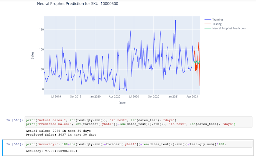
layout = go.Layout(title=('Neural Prophet Prediction for SKU: '+ str(sku)), xaxis=dict(title='Date'), yaxis=dict(title='Sales'))
fig = go.Figure(data=[daily_sales_train,daily_sales_test,daily_sales_pred], layout=layout)
iplot(fig)
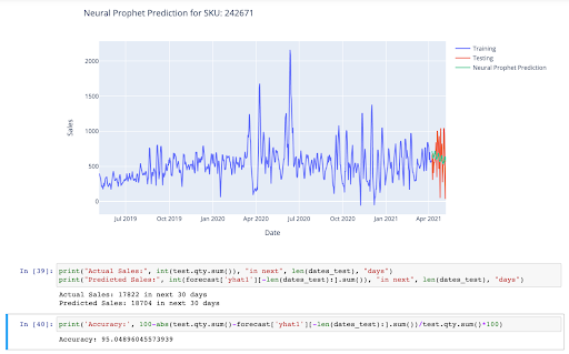
            print("Actual Sales:", int(test.qty.sum()), "in next", len(dates_test), "days")
            print("Predicted Sales:", int(forecast['yhat1'][-len(dates_test):].sum()), "in next", len(dates_test), "days")
print('Accuracy:', 100-abs(test.qty.sum()-forecast['yhat1'][-len(dates_test):].sum())/test.qty.sum()*100)
This forecasting model can produce extremely accurate results, for even as long as 90 days into the future. When the parameters - yearly seasonality, selling price, etc. are rightly set, the model can easily produce results with less than 10% error. Without SKU information, and trial and error, the accuracy can vary from as low as 40% to as high as 98%. Therefore, the parameters need to be rightly set before the prediction is made.
The model also provides insights into various seasonalities which can be used to draw important conclusions and plan out promotional offers or discounts on products.


Currently, the model has been built to be able to use selling price as an input feature and a future regressor. Other relevant data such as promotional offers, or COVID cases can also be built into the model similarly.